Statistical Tests

the multicompare function can run repeated statistical test across a features (genes). It requires to select a list of groups to be compared, and a one-hot-encoded matrix with groups membership. If only two groups are provided, Mann-Whitney U test [Mann1947] will be run, if more, a Kruskal-Wallis H test [Kruskal1952] will be used instead. A data dataframe matrix containing the values to compare (e.g. TMM-normalized counts obtained with edger.build_dgelist) needs to be provided.

The output genes can be filtered through a p-value cutoff, while further flags like which method to use (multi_method) and the \({\alpha}\) (multi_alpha) can be provided for the multiple testing correction.

from tapir.stats import multicompare

stats, dunn = multicompare(groups, membership, data,
      cutoff=1, multi_method='fdr_tsbh', multi_alpha=0.05)

In output is a dataframe with median values, ratio, difference and p-values for each provided genes. If Kruskal-Wallis was selected, the Dunn post-hoc test [Dunn1961] results are also provided.

Contingency tables

Contingency tables can be built and related tests can be run with TAPIR.

form tapir.stats import get_contingency, test_contingency

contab = get_contingency(series, groups, membership)
stats  = test_contingency(contab, method='auto')

The get_contingency function requires a series containing the variable to evaluate (e.g. sex, therapy status, mutation), the groups to compare and the one-hot-encoded membership table. The significance of the resulting table can be then measured with test_contingency. This will automatically select between Fisher exact test [Fisher1992] if a 2x2 matrix is provided or a \({\chi^2}\) test [Pearson1900] otherwise, but each method can be manually chosen. If the \({\chi^2}\) test is selected and insufficient populations are provided, the function will throw a warning and return None.

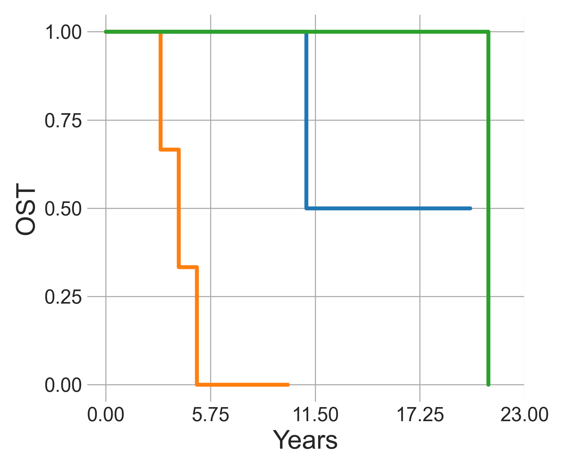
Survival lines

Survival analysis is available through lifelines. For now, only Kaplan-Meier fitted curves, and log-ratio are available.

The survival data (st_stats) needs to be formatted as a pandas dataframe with the time value in survival_times and a binary death event observation in event_observed.

As for other functions, a list of groups to be compared needs to be provided, together with a one-hot-encoded matrix with groups membership.

from tapir.stats import st_curves
from tapir.plotting import plot_survival

stats, curves = st_curves(st_stats, groups, membership)
plot_survival(curves, xlab='Years', ylab='OST', save_file='./plot.png')

The resulting p-value can be found in stats, while curves can be plotted with plot_survival.

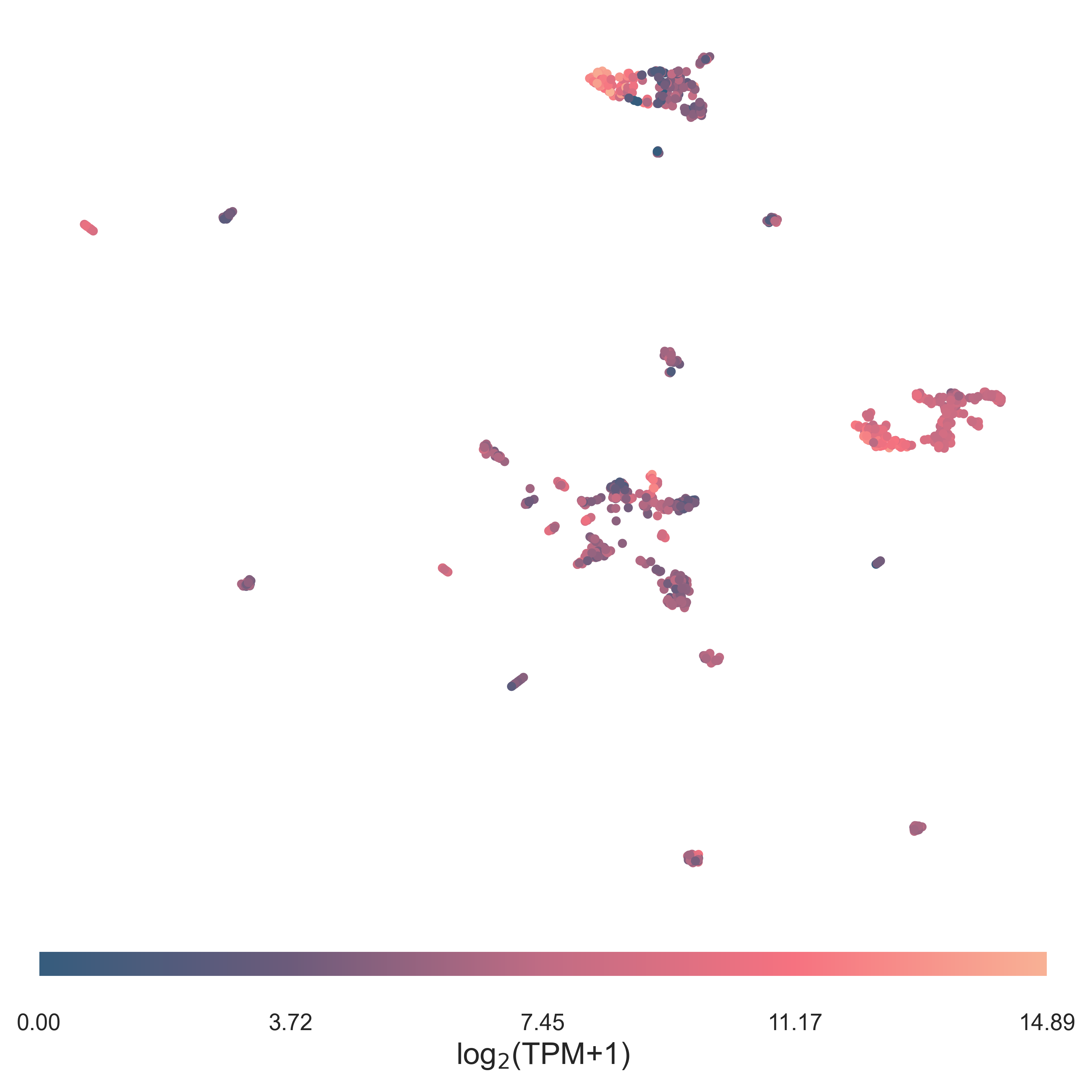
Dimensionality reduction

TAPIR provides a quick interface for dimensionality reduction with umap and plotting its results. get_umap only takes the data to be mapped (e.g. expression counts), with samples as rows and features as columns. The var_drop_thresh cutoff can be provided for low variance removal. The most variant genes whose variance sum up to the given threshold percentage will be kept. Alternatively collinear_thresh collinearity can be removed by providing a correlation threshold, albeit the current implementation is particularly slow and not recommended. UMAP will be run with preselected settings, but these can be adjusted by providing the appropriate UMAP object keywords.

from tapir.embedding import get_umap
from tapir.plotting import plot_clusters

proj, mappa = get_umap(data, collinear_thresh=None, var_drop_thresh=.99)
proj.index  = data.index

plot_clusters(proj, groups=None, values=data['MYCN'], clab='log$_2$(TPM+1)',save_file='./map.png')

Continuous values can be provided as colormap when plotting. Alternatively if a list of groups is provided, the datapoints will be coloured accordingly.

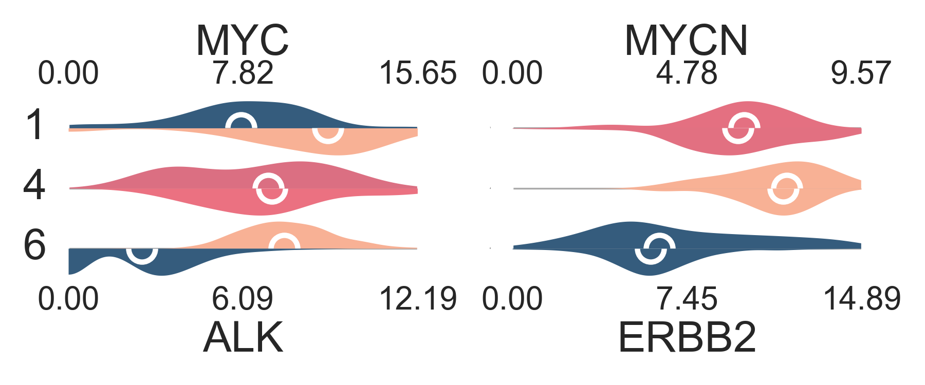
Other plots

The expression values or gene set enrichment scores can be plotted as distributions using plot_distribution. Groups and membership table need to be provided. This function allows to plot on one (genes_up) or two levels (if genes_dw is also provided) for an easy comparison.

from tapir.plotting import plot_distribution

plot_distribution(data, groups, membership,
  genes_up, genes_dw,
  save_file='./distribution.png')

Similarly, the median values can be plotted as a heatmap with plot_heatmap

from tapir.plotting import plot_heatmap

plot_heatmap(data, groups, membership, genes,
  clab='log$_2$(TPM+1)',
  save_file='./heatmap.png')

Labels and color map range can be customized to a degree. For the full list of available options and their use, see API.

References

Mann1947: Mann, H. B., Whitney, D. R. (1947). “On a Test of Whether one of Two Random Variables is Stochastically Larger than the Other”, Annals of Mathematical Statistics. 18 (1): 50–60.
Kruskal1952: Kruskal W. H., Wallis W. A. (1952). “Use of ranks in one-criterion variance analysis”, Journal of the American Statistical Association. 47 (260): 583–621.
Dunn1961: Dunn O. J. (1961). “Multiple Comparisons among Means”, Journal of the American Statistical Association, 56:293, 52-64.
Fisher1992: Fisher R. A. (1992). “Statistical Methods for Research Workers”, In: Kotz S., Johnson N.L. (eds) “Breakthroughs in Statistics”. Springer Series in Statistics (Perspectives in Statistics). Springer, New York, NY.
Pearson1900: Pearson, K. (1900). “On the criterion that a given system of deviations from the probable in the case of a correlated system of variables is such that it can be reasonably supposed to have arisen from random sampling”, The London, Edinburgh, and Dublin Philosophical Magazine and Journal of Science, 50(302), 157–175.